周次: 7 备注: Attendance check 日期: April 8, 2022 节次: 2

In this lecture, we will take a quick glance at the Numerical Integration methods. Numerical integrations are very useful in practice. The methods we are going to learn are Trapezoidal Method and Simpson’s Method. We will learn how to evaluate an integration numerically, and how to predict the error the evaluation produces.

General Thoughts on Numerical Integrations

Riemann Sum Provides a Good Approximation Indeed

As evaluate a definite integral, we have seen that by subdividing the interval into several sub-intervals, we obtained a Riemann sum to the integration

$$ \sum_{i=1}^n f(\xi_i)\Delta x_i\approx \int_a^b f(x)dx. $$

The approximation has been approved by the definition of the definite integral. And we have shown by an example that as the mesh becomes finer and finer, the approximation is getting more and more accurate.

An integrable function does not constrain on how the meshes should be looked like. For our convenience, we make the subdivision evenly spaced. In this case, the Riemann sum is getting even more simplified

$$ (b-a) \dfrac{\sum_{i=1}^n f(\xi_i)}{n}. $$

That is, an average of $n$ samples $f(\xi_i)$, multiplying the length of the interval.

So in principal, numerical integration is as easy as sampling and averaging. A crazier idea for numerical integration is called Monte Carlo Integration.

Monte Carlo Integration

To integrate a function $f(x)$ from $a$ to $b$, we could blindly (randomly) choose $n$ sampling points, evaluate the function at those points, and take an average. If the sampling is uniformly distributed, the average will eventually become a good approximation of the integration. (By applying the central limit theorem in statistics.)

$$ \int_a^b f(x) dx \approx \frac{b-a}{n}\sum_{i=1}^n f(r_i) $$

where $r_i$ is randomly chosen (with equal probability everywhere) sampling point inside of the interval $[a,b].$

Trapezoidal Approximations

The Trapezoidal rule for the value of a definite integral is based on approximating the region between a curve and the $x$-axis with trapezoids instead of rectangles. It is not necessary for the subdivision points $x_0$, $x_1$, $x_2,$ $\cdots$, $x_n$ to be evenly spaced, but the resulting formula is simpler if they are.

Assuming the length of each subinterval is

$$ \Delta x = \frac{b-a}{n}. $$

It is called the step size or mesh size. The area of the trapezoid that lies above the $i$th subinterval is

$$ \Delta x \left(\dfrac{y_{i-1}+y_i}{2}\right) = \dfrac{\Delta x}{2}\left(y_{i-1}+y_i\right) $$

where $y_i = f(x_i)$.

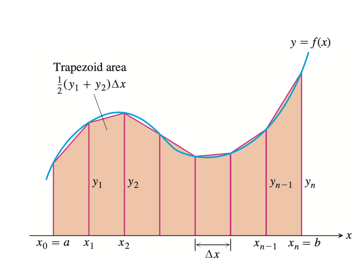
So the area below the curve is approximated by

$$ T = \frac{1}{2}(y_0+y_1)\Delta x + \frac{1}{2}(y_1+y_2)\Delta x + \cdots + \frac12 (y_{n-1}+y_n)\Delta x \ = \frac{\Delta x}{2}\left(y_0 + 2 y_1 + 2y_2 +\cdots + 2y_{n-1} + y_n\right) $$

where

$$ y_0 = f(a),\quad y_1 = f(x_1),\quad \cdots \quad y_{n-1} = f(x_{n-1}),\quad y_n = f(b). $$

The Trapezoidal Rule

To approximate $\int_a^b f(x)dx,$ use

$$ T = \frac{\Delta x}{2}\left(y_0+2y_1 + 2y_2 + \cdots + 2y_{n-1} + y_n\right). $$

The $y$’s are the values of $f$ at the partition points $x_k = a + k \Delta x$, where $\Delta x = \frac{b-a}{n}$.

Example 1. Applying the Trapezoidal Rule

Use the Trapezoidal rule with n=4 to estimate $\int_1^2 x^2 dx$. Compare with the exact value.

Solution.

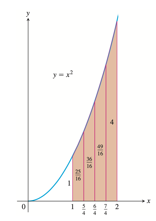
$$ T = \frac{\Delta x}{2}\left(1 + 2 \cdot \frac{25}{16} + 2 \cdot \frac{36}{16} + 2\cdot \frac{49}{16} + 4\right) = \dfrac{75}{32} = 2.34375 $$

And the exact value is $7/3$. The $T$ approximation overestimates the integral by about $0.446%$. The overestimation is expected, due to the curve being concave up.

We would also expect that a rectangle estimation on the same meshes will produce larger error.

Example 2. Averaging Temperatures

An observer measures the outside temperature every hour from noon until midnight, recording the temperatures in the following table.

Time	N	1	2	3	4	5	6	7	8	9	10	11	M
Temp	63	65	66	68	70	69	68	68	65	64	62	58	55

What was the average temperature for the 12-hour period?

Solution. We are looking for the average value of a continuous function (temperature). We need to find

$$ \text{av}(f) = \frac{1}{b-a}\int_a^b f(x) dx, $$

without knowing a formula for $f(x)$. The integral can be approximated by the Trapezoidal rule.

$$ T = \frac{\Delta x}{2}\left(y_0 + 2y_1 + 2y_2 + \cdots + 2y_{11} + y_{12}\right)\ = \frac12 \left(63 + 2\times 65 + 2\times 66 + \cdots + 2\times 58 + 55\right)=782. $$

Therefore, $\text{av}(f)\approx \frac{1}{b-a}T = 782/12\approx 65.17.$

Error Estimates for the Trapezoidal Rule

The $T$ approaches the exact integral $\int_a^b f(x)dx.$ Since

$$ T = \Delta x \left(\frac12 y_0 + y_1 + y_2 + \cdots + y_{n-1} + \frac12 y_n\right)\ = (y_1 + y_2 + \cdots + y_n )\Delta x + \frac12 (y_0-y_n)\Delta x \= \sum_{k=1}^n f(x_k)\Delta x + \frac12 \left[f(a)-f(b)\right]\Delta x. $$

As $n\to \infty$ and $\Delta x\to 0,$ we can clearly see that $\lim_{n\to\infty} T = \int_a^b f(x) dx.$

In practice, we want to know how fast the Trapezoidal method converges to the exact value, or how large $n$ should be for a given tolerance?

RESULT. The error estimation

If $f''$ is continuous on $[a,b]$, then

$$ ｜E_T ｜:= \left|\int_a^b f(x)dx - T\right|\le \dfrac{b-a}{12}\max |f''(x)| (\Delta x)^2 $$

If we substitute $\frac{b-a}{n}$ for $\Delta x$, and an upper bound $M$ for the $|f''(x)|$ on $[a,b]$, we get

$$ |E_T|\le \dfrac{M(b-a)^3}{12n^2} $$

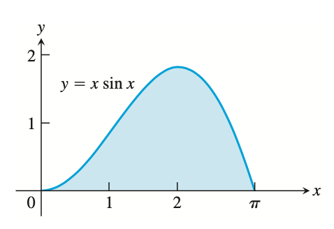
Example 3. Bounding the Trapezoidal Rule Error

Find an upper bound for the error incurred in estimating

$$ \int_0^\pi x \sin x dx, $$

with the Trapezoidal Rule with $n=10$ steps.

Solution. Since

$$ |f''(x)| = |2\cos x - x\sin x|\le 2 |\cos x| + |x||\sin x|\le 2 + \pi $$

The error

$$ |E_T| \le \frac{\pi^3}{1200} M = \frac{\pi^3(2+\pi)}{1200}< 0.133. $$

For greater accuracy, we would increase the number of steps. As we can see for $n=100$ steps, the error is no more than $1.33\times 10^{-3}$.

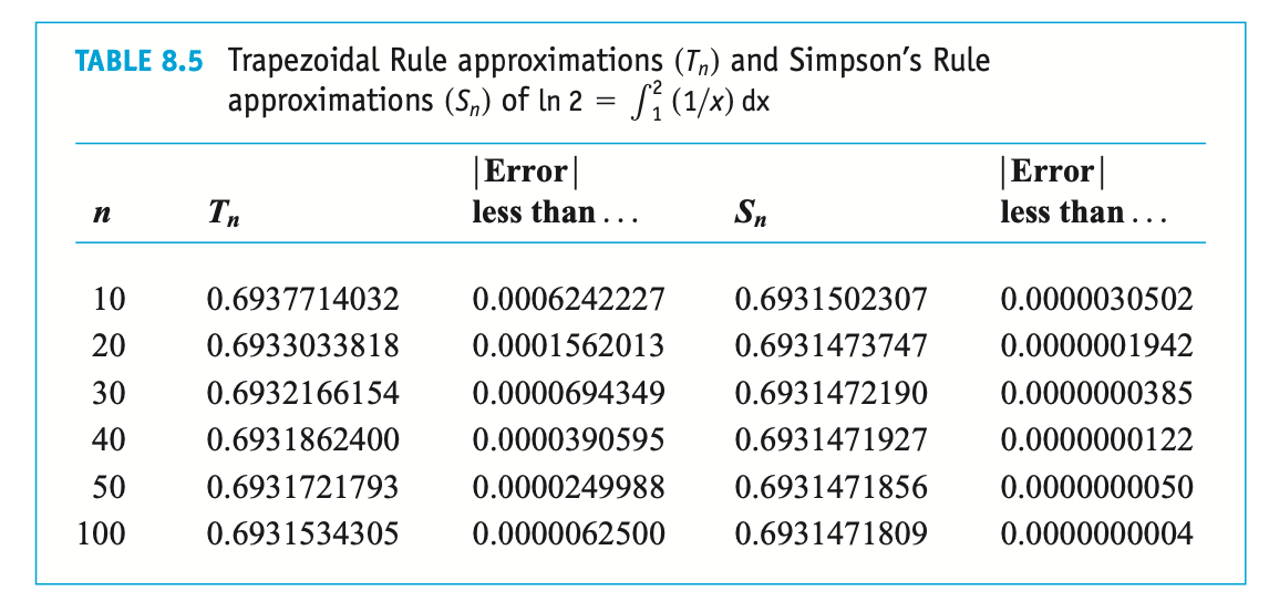
Example 4. Finding How Many Steps Are Needed For a Specific Accuracy

How many subdivisions should be used in the Trapezoidal Rule to approximate

$$ \ln 2 = \int_1^2 \frac1x dx, $$

with a tolerance less than $10^{-4}.$

Solution. For function $f=1/x$, the upper bound for $f''$ on the interval $[1,2]$ is $2$. Hence

$$ |E_T|\le \frac{(2-1)\times 2}{12 n^2}=\frac{1}{6n^2}. $$

In order to make error less than $10^{-4},$ we need $\frac1{6n^2}<10^{-4}$, or $n>40.83.$

Simpson’s Rule: Approximations Using Parabolas

Instead of using trapezoidal shapes for defining the area, we now use the shaded area beneath a parabola passing through three consecutive points. As illustrated in the following graph.

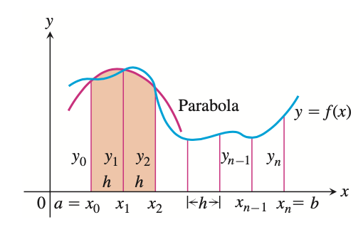
To obtain an estimation, we subdivide the interval $[a,b]$ into $n$ subintervals of equal length $h =\Delta x = \frac{b-a}{n}$, but this time we require that $n$ be an even number.

On each consecutive pair of intervals we approximate the curve $y=f(x)$ by a parabola, passing through consecutive points $(x_{i-1},y_{i-1})$, $(x_i,y_i)$ and $(x_{i+1},y_{i+1})$ on the curve.

To compute the shaded area, let’s move the $y$-axis to $x=x_i$ (which does not change the area). Suppose the parabola has the form $Ax^2+Bx + C$, then the area will be

$$ A_p = \int_{-h}^h (A x^2 + B x + C) dx = \frac{h}{3}\left(2A h^2 + 6C\right). $$

Since the parabola is passing through points $(-h,y_{0})$, $(0,y_1)$ and $(h,y_2)$, we can solve the equation to find

$$ C = y_1,\quad 2A h^2 = y_0+y_2 - 2y_1 $$

Therefore the area $A_p$ is

$$ A_p = \frac{h}{3} (y_0 + 4 y_1 + y_2). $$

Then approximating the integral $\int_a^b f(x)dx$ obtains the following formula

$$ \int_a^b f(x)dx \ \approx \frac{h}{3}(y_0 + 4y_1 + y_2) + \frac{h}{3}(y_2+4y_3 + y_4) + \cdots + \frac{h}{3}(y_{n-2}+4y_{n-1} + y_n)\ = \frac{h}{3}\left(y_0 + 4y_1+2y_2 + 4y_3 + 2 y_4 +\cdots + 2y_{n-2}+4y_{n-1}+y_n\right) $$

Simpson’s Rule

To approximate $\int_a^b f(x)dx,$ use

$$ S=\frac{\Delta x}{3}(y_0+4y_1 + 2y_2 + 4y_3 + \cdots + 2y_{n-2} + 4y_{n-1} + y_n). $$

The $y$’s are the values of $f$ at the partition points $x_k = a + k \Delta x$. And $n$ is even, $\Delta x = (b-a)/n.$

Note the pattern of the coefficients in Simpson’s rule: $1, 4, 2, 4, 2, \cdots, 2,4, 1$.

Example 5. Applying Simpson’s Rule

Use Simpson’s Rule with $n=4$ to approximate $\int_0^2 5x^4 dx$.

Solution. Partition $[0,2]$ into four subintervals, then $\Delta x = \frac12.$

$$ S = \frac{\Delta x}{3}\left(y_0 + 4 y_1 + 2y_2 + 4y_3 + y_4\right)=32\frac{1}{12} $$

The exact value is $32$.

Error Estimates for Simpson’s Rule

If $f^{(4)}$ is continuous and $M$ is any upper bound for the values of $|f^{(4)}|$ on $[a,b]$, then the error $E_S$ in the Simpson’s Rule approximation satisfies

$$ |E_S|\le \dfrac{M(b-a)^5}{180 n^4}. $$

Example 6. Bounding the Error in Simpson’s Rule

Find an upper bound for the error in estimating $\int_0^2 5x^4 dx$ using Simpson’s Rule with $n=4$.

Solution. Since $f^{(4)}(x) = 120$. We take $M=120$, with $b-a=2$ and $n=4$, the error is no more than

$$ |E_S|\le \frac{120 \times 2^5}{180 \times 4^4}=\frac1{12} $$

Example 7. Comparing the Trapezoidal’s and Simpson’s Rules

Notice that if $f(x)$ is a polynomial of degree less than $4$, then $f^{(4)}$ is zero, and Simpson’s rule shows no error no matter how many steps. Similarly, for constant or linear functions, the $f''$ is zero, therefore the Trapezoidal rule shows no error.

Example 8. Estimate

$$ \int_0^2 x^3 dx $$

with Simpson’s Rule.

Solution. Indeed, with $n=2$ and $\Delta x = 1$, we find

$$ S = \frac{1}{3}(y_0+4y_1+y_2) = 4 $$

which is exactly the value of integration.

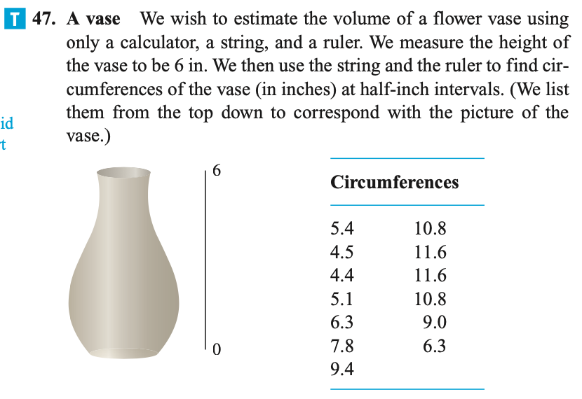
Example 9. A Real Case